1 Overview

Please start by logging into sso.rstudio.cloud/pomona. Once you’ve logged in, you should see the option to open the EA 30.1 - Fall 2022 workspace. You can also access the EA 30.1 - Fall 2022 workspace at this link.

At the workspace, you should then see the “Assignment” Acoustics. Please click on that Assignment. Here is a direct link to the Acoustics project, but it may not work if this is the first time in a while that you’re logging into RStudio.Cloud. If it doesn’t work, no worries - just log in through the sso.rstudio.cloud/pomona link.

In this tutorial, we’ll take a look at sound data collected at the Bernard Field Station this past October, or earlier this year.

In this tutorial, you will learn:

what are different ways to interact with sound data in R?
how can we visualize sound data using spectrograms?
how can we calculate indices of acoustic diversity?

2 A brief description of sound

When we vocalize, we are making vibrations that move through the air like a wave. Microphones detect these vibrations. These vibrations are then recorded into numbers which can be processed by computers. It turns out that we can get quite a bit of information from these numbers.

Let’s start by loading the packages that we will need.

### Loading packages
library(seewave)
library(tuneR)
library(dplyr)
library(readr)

2.1 Waveforms

Let’s pull in one of the recorded files from the BFS. You can play the recording below.

Now, let’s visualize this recording using an oscillogram. The output from the function oscillo shows how how the amplitude (or loudness) changes over the whole recording. We’re going to focus on visualizing the recording from 0:00 to 0:05

## Read in the sound data
BFS_am_1 <-tuneR::readWave('20221103_062700.WAV')

## Show the oscillogram
## which is a plot of amplitude over time
oscillo(BFS_am_1, from=0, to= 5, fastdisp=TRUE)

One thing to note is that these data were recorded at a frequency of 48,000 records per second. So even though each sound file is only 30 seconds long, it has a total of 1,440,000 data points! (This is equal to 30 seconds / minute * 48000 records/second.)

2.2 Spectrogram

Another way that we can visualize sound is to use the fact that sound has the property of frequency (pitch) at particular times. We can also include amplitude (loudness) as a color. A spectrogram let’s us display all three elements of an acoustic signal: its time/duration, the frequency (pitch) of the sound, and the loudness of the sound at each frequency (pitch).

We see that the frequencies in this sound recording are mostly located from 0 to 5000 Hz (or 5 kHz).

## Use spectro to display the spectogram of this data
spectro(BFS_am_1, fastdisp=TRUE)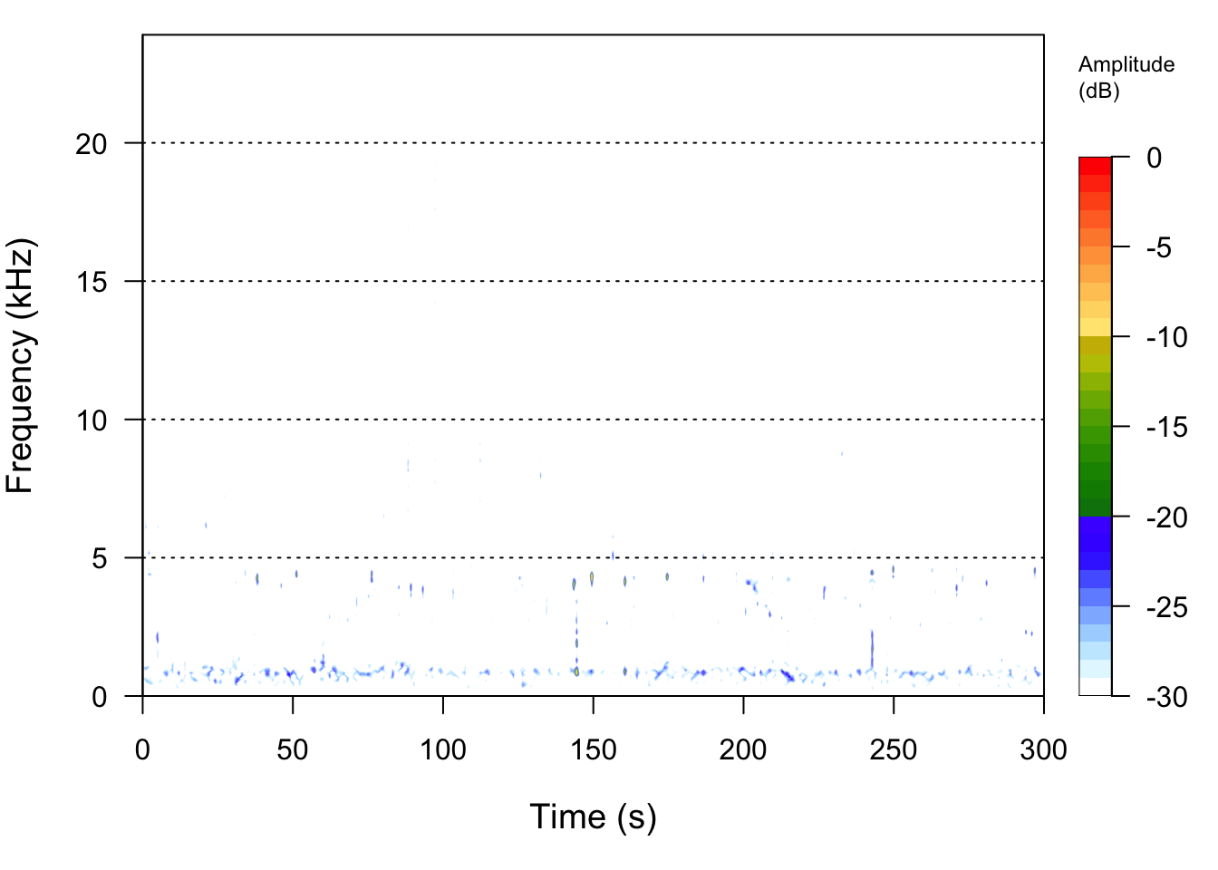

  # NB: you may need to make the plotting window larger

3 Soundscape indices

From observational data of species, we can calculate metrics such as species richness, Shannon’s index, etc. Similarly, from sound data, we can calculate metrics of acoustic complexity, which theoretically should be related to the overall biodiversity of vocalizing animals.

First, let’s now also read in an evening recording.

## Read in the sound data for the evening
BFS_pm_1 <-tuneR::readWave('20221020_191500.WAV')

Here, we will use the function ACI to calculate the acoustic complexity of a morning versus evening recording from the BFS.

ACI(BFS_am_1)

## [1] 150.2826

ACI(BFS_pm_1)

## [1] 167.0415

4 Processed data

In addition to using numeric metrics such as ACI to calculate the acoustic diversity of audio recordings, we can use new computer vision models to identify (bird) species in the recordings. We have and will process/ed the raw recording data to:

Calculate ACI for each 30 second recording - in progress; to be done for the class recordings
Identify bird vocalizations in each 30 second recording - complete; to be done for the class recordings

We have used Cornell Lab of Ornithology’s BirdNET neural network model, which is trained on data such as identified acoustic recordings from xeno-canto. This model extracts distinct bird vocalizations from the spectrographic representation of each sound file. Those bird vocalizations are then pattern matched against known bird vocalizations to generate the most likely species (of the 3000 species supported by the model) with some probability (a.k.a. confidence).

Let’s take a look at the data.

# Read in a spreadsheet from a URL using read_tsv from the readr package
birdnetDF <- readr::read_tsv("https://github.com/EA30POM/site/raw/main/data/birdnet10-22.tsv")

## Parsed with column specification:
## cols(
##   Selection = col_double(),
##   View = col_character(),
##   Channel = col_double(),
##   BeginTimeS = col_double(),
##   EndTimeS = col_double(),
##   LowFreqHz = col_double(),
##   HighFreqHz = col_double(),
##   SpeciesCode = col_character(),
##   CommonName = col_character(),
##   Confidence = col_double(),
##   unit = col_character(),
##   date = col_date(format = ""),
##   time = col_character(),
##   DayNight = col_character()
## )

# Inspect the data
birdnetDF %>% head() # look at the first 6 rows

## # A tibble: 6 x 14
##   Selection View    Channel BeginTimeS EndTimeS LowFreqHz HighFreqHz SpeciesCode
##       <dbl> <chr>     <dbl>      <dbl>    <dbl>     <dbl>      <dbl> <chr>      
## 1         1 Spectr…       1          0        3       150      12000 caltow     
## 2         2 Spectr…       1          3        6       150      12000 caltow     
## 3         3 Spectr…       1          6        9       150      12000 caltow     
## 4         4 Spectr…       1          9       12       150      12000 caltow     
## 5         5 Spectr…       1         12       15       150      12000 caltow     
## 6         6 Spectr…       1         15       18       150      12000 caltow     
## # … with 6 more variables: CommonName <chr>, Confidence <dbl>, unit <chr>,
## #   date <date>, time <chr>, DayNight <chr>

Below, I’ll walk you through some possible analyses with the BirdNET identifications, so that this can be grist for the mill for thinking about a hypothesis that your group can take on. Let’s start by removing low confidence recordings (e.g. confidence \[ < 0.5\]).

# Filter out low confidence identifications
birdnetDF <- birdnetDF %>%
  dplyr::filter(Confidence >= 0.5) # only retain the rows (observations) where Confidence >= 0.5

Now, let’s say that we were interested in evaluating the number of species identified during the day or night. How would we do that?

# Analyzing number of species during the day or night
birdnetDF %>%
  group_by(DayNight) %>% # group by the Day or Night categories
  summarize(NumSpecies = length(unique(CommonName))) # number of distinct species per category

## `summarise()` ungrouping output (override with `.groups` argument)

## # A tibble: 2 x 2
##   DayNight NumSpecies
##   <chr>         <int>
## 1 Day             195
## 2 Night           144

Below is a summary of what the relevant columns in the class data are or will be:

birdnet Data:

SpeciesCode: A six letter short-hand code for species, determined by groups such as the American Ornithological Society
CommonName: The common name for different species identified in each 3 second window of the recording
Confidence: The confidence of the identification for each species in each 3 second window
unit: Which unit recorded the data
date: What was the date of the recording?
time: What was the time of the recording?
DayNight: Was the recording made during the daytime or nighttime?

ACI Data (forthcoming):

Many of the columns will be the same as the birdnet data, though some column names may be capitalized (e.g. Unit instead of unit).

ACI: the acoustic complexity index value for each 30 second recording.

Each of your groups is required to submit 3 hypotheses by the end of Week 3 of this lab (Week 13 of class). Please confer with your groups on possible hypotheses that you can explore with these data. Some additional variables beyond the bird identification or ACI variables that we can obtain as a class include:

Precipitation
Temperature
Time of year (date)
BirdCast migration estimates for Los Angeles County (see the Birds in flight (nightly avg.) plot FMI)
Habitat type in the BFS (determined by the unit’s location)
Distance to road or edge of the BFS (determined by the unit’s location)
… other variables that you may think of and are feasible for us to collect!

5 `R` script

Below is the R script in its entirety.

### Loading packages
library(seewave)
library(tuneR)
library(dplyr)
library(readr)

## Read in the sound data
BFS_am_1 <-tuneR::readWave('20221103_062700.WAV')
## Show the oscillogram
## which is a plot of amplitude over time
oscillo(BFS_am_1, from=0, to= 5, fastdisp=TRUE)

## Use spectro to display the spectogram of this data
spectro(BFS_am_1, fastdisp=TRUE)
    # NB: you may need to make the plotting window larger

## Read in the sound data for the evening
BFS_pm_1 <-tuneR::readWave('20221020_191500.WAV')

### ACI - acoustic complexity index calculations
ACI(BFS_am_1)
ACI(BFS_pm_1)

# Read in a spreadsheet from a URL using read_tsv from the readr package
birdnetDF <- readr::read_tsv("https://github.com/EA30POM/site/raw/main/data/birdnet10-22.tsv")

# Inspect the data
birdnetDF %>% head() # look at the first 6 rows

# Filter out low confidence identifications
birdnetDF <- birdnetDF %>%
  dplyr::filter(Confidence >= 0.5) # only retain the rows (observations) where Confidence >= 0.5

# Analyzing number of species during the day or night
birdnetDF %>%
  group_by(DayNight) %>% # group by the Day or Night categories
  summarize(NumSpecies = length(unique(CommonName))) # number of distinct species per category

Acoustic ecology - studying environments through sound