Week 3
2024-09-17
1 Preparing data and accessing RStudio Server
Please start by logging into rstudio.pomona.edu.
1.1 Load packages
Below, we will start by loading packages that we’ll need. Remember,
you may need to run install.packages('PACKAGENAME') just
once this semester if you get an error for a particular package.
### Load packages
library("ggplot2") # plotting functions
library("dplyr") # data wrangling functions
library("tidyr") # data wrangling functions
library("readr") # reading in tables, including ones online
library("lubridate") # a package to specify date-time stamps
library("mosaic") # shuffle (permute) our data
1.2 Read data
Next, we will pull in our data.
### Load in dataset
temperature_data <- readr::read_csv("https://github.com/EA30POM/site/raw/main/data/temperature-c.csv")
pm25_data <- readr::read_csv("https://github.com/EA30POM/site/raw/main/data/us-epa-pm25-aqi_claremont.csv")

### How many observations and columns do we have?
dim(temperature_data)
1.2.1 Using the
View command
Oftentimes, we may want a more intuitive way to see our data tables.
It can be really annoying when R is too clever and only
displays a subset of the columns of your spreadsheet. The
View() function pulls up an Excel-style data viewer. Let’s
try it below:
View( head( temperature_data ) )1.3 Cleaning the data
Below, we are going to modify some of the data attributes to be able to seamlessly join these two variables together.
# Clean the DateTime column using lubridate's ymd_hms function
temperature_data <- temperature_data %>%
  mutate(DateTime = lubridate::ymd_hms(DateTime))

pm25_data <- pm25_data %>%
  mutate(DateTime = lubridate::ymd_hms(DateTime))
Now, we are going to cast these data to a “long” format (each row is an individual observation only) so that we can more easily match across datasets.
# Convert the temperature_data to a long format
temperature_long <- temperature_data %>%
  tidyr::pivot_longer(cols = -DateTime, names_to = "Station", values_to = "Temperature")  %>%
  dplyr::distinct(DateTime, Station, .keep_all = TRUE)

# Convert the pm25_data to a long format
pm25_long <- pm25_data %>%
  tidyr::pivot_longer(cols = -DateTime, names_to = "Station", values_to = "PM2_5") %>%
  dplyr::distinct(DateTime, Station, .keep_all = TRUE)
Now we are ready to join our data! We are going to join based on
matching values for Station and DateTime.
# Merge the temperature and pm25 data by DateTime and Station
airDF <- inner_join(temperature_long, pm25_long, by = c("DateTime", "Station"))

# Create separate columns for Date and Time
airDF <- airDF %>%
  mutate(
    Date = as.Date(DateTime),          # Extract the date
    Time = format(DateTime, "%H:%M:%S") # Extract the time in HH:MM:SS format
  )
I’m going to use the pipe operator %>% to daisy chain
commands together into a sequence. It is a handy way to make a complex
operation with intermediate steps more transparent. The visualization
below describes what pipes do in R in linking up
functions:
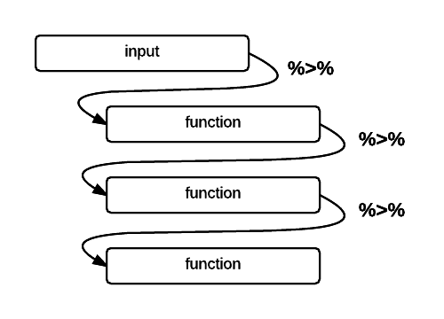
%>%
operator in R (Altaf Ali)airDF %>% head() %>% View()1.3.1 Pre-processing the data
Now we’ll use that handy %>% operator to clean our
data. We’ll also use a very helpful function called mutate.
mutate is a command to either alter an existing column or
create a new column in the data.
### Pre-processing steps
  # We want the Date and Time columns to be datetime objects
airDF <- airDF %>%
  mutate(Date = lubridate::ymd(Date), Time=lubridate::hms(Time))
  # We want to code which observations are made in the day vs. night
  # using 6pm as our cut-off
pm_limit <- lubridate::hms("18:00:00")

### Add on a new column to note whether or not the data is day or night
airDF <- airDF %>%
  mutate(DayNight = case_when( Time >= pm_limit ~ "Night",
                               TRUE ~ "Day"))

### Remove rows with missing values
airDF <- tidyr::drop_na(airDF)
2 Analyzing the data
Below, I provide fully-worked examples of different ways of
inspecting your data and performing analyses assuming that
PM2_5 is the variable of interest. In applying
this code to your own data, you will want to think about what variable
name should replace PM2_5 in the commands
below.
Let’s start with exploratory data analysis where you calculate
summary statistics and visualize your variable. Let’s say that I’m
interested in understanding how the values of PM2.5 (PM2_5)
vary across day and night (a silly example, I know). We’ll use another
function: group_by splits a data table into groups based on
distinct values a variable that has categories. In this
case, we tell group_by to divide up the airDF
data table into groups based on the values of DayNight. We
then will use a function summarize to get summary
statistics of PM2_5 in the day and night.
### Calculate summary statistics for PM2_5
### for each DayNight condition
airDF %>%
  group_by(DayNight) %>%
  summarize(min=min(PM2_5,na.rm=T), mean=mean(PM2_5,na.rm=T), max=max(PM2_5,na.rm=T))
  # use DayNight as the grouping variable
  # for PM2_5 and then summarize PM2_5
  # for each value of DayNight and pass in the parameter
  # na.rm=T to ignore missing values
2.1 Do day and night differ in their PM2.5 levels?
How do PM2.5 levels vary across day and night? We can visualize that using a boxplot. Boxplots are useful for depicting how different discrete categories within a variable exhibit variation. Below, we will specify the variable that we use to group our data (Day/Night) as the x variable, and the values of interest as the y variable (PM2_5, or PM2.5).
p <- ggplot(airDF, aes(x=DayNight, y=PM2_5))
p <- p + geom_boxplot()
p <- p + labs(x="",y="PM2.5 (PM2_5)")
p <- p + theme_minimal()
p
Let’s calculate the difference between Day and Night in terms of
their mean PM2_5 values.
### Calculating differences in mean PM2_5 values
obs_diff <- diff( mean( PM2_5 ~ DayNight, data=airDF, na.rm=T ) )
obs_diff # print out the value
OK, so we see that there is a difference in mean PM2.5 levels across day and night. Is this a meaningful difference though? Our null hypothesis is that there is no difference in mean PM2.5 levels between day and night (again, a silly example, I know).
Logically, if there is a meaningful difference, then if we shuffle our data around, that should lead to different results than what we see. That is one way to simulate statistics to test the null hypothesis. And specifically, in this case, we would expect to see our observed difference is much larger than most of the simulated values.
What does simulating our data look like?
Well, here is what the data look like initially. We’re going to use
another function, select, to pull out particular columns of
interest from the data.
airDF %>%
  dplyr::select(Date,Time,PM2_5,DayNight)
Here’s what the data look like if we shuffle it by randomizing the
assignment of observations as day or night. This is like a chaos agent
coming around and slapping a new label for day or night on at random for
every row in the data table. (But if we think mean(PM2_5)
is the same for Day and Night, then that
should be a perfectly OK action by the chaos agent.)
print(resample(airDF[,c("Date","Time","PM2_5","DayNight")],groups=DayNight,shuffled=c("PM2_5")))We can repeat that procedure again and see how the data shifts if we do another shuffle.
print(resample(airDF[,c("Date","Time","PM2_5","DayNight")],groups=DayNight,shuffled=c("PM2_5")))Let’s shuffle the data and see what that means for the distribution
of mean PM2_5 differences between day and night.
### Create random differences by shuffling the data
randomizing_diffs <- do(1000) * diff( mean( PM2_5 ~ shuffle(DayNight),na.rm=T, data = airDF) ) # calculate the mean in PM2_5 when we're shuffling the day/night values around 1000 times
  # Clean up our shuffled data
names(randomizing_diffs)[1] <- "DiffMeans" # change the name of the variable

# View first few rows of data
head(randomizing_diffs)
Now we can visualize the distribution of simulated differences in mean PM2.5 levels. Where would our observed difference in mean light levels fall?
gf_histogram(~ DiffMeans, fill = ~ (DiffMeans <= obs_diff),
             data = randomizing_diffs,
             xlab="Difference in mean PM2.5 across day/night under null",
             ylab="Count")
In the end, how many of the simulated mean differences were larger than the value we observed? Based on this value, if we were using the conventional \(p\)-value (probability value) of 0.05, we would conclude that because this simulated \(p\)-value < 0.05, that we reject the null hypothesis. There is a difference in mean PM2.5 level between day and night.
# What proportion of simulated values were larger than our observed difference?
prop( ~ DiffMeans <= obs_diff, data = randomizing_diffs)
2.2 Calculating correlations between numeric variables
Let’s say that instead of comparing PM2.5 across day and night, I want to compare PM2.5 against temperature. PM2.5 and temperature are both numeric variables. There aren’t obvious categories for either variable.
What do these two variables look like? What does the potential relationship between them look like? We can use a scatterplot to find out.
p <- ggplot(airDF, aes(x=Temperature, y=PM2_5))
p <- p + geom_point()
p <- p + labs(x="Temperature (*C)",y="PM2.5 (PM2_5)")
p <- p + theme_bw()
p
If I’m interested in seeing if
lower temperature is associated with lower (or higher) PM2.5 levels.
I can measure that by calculating a correlation coefficient.
### Calculate observed correlation
obs_cor <- cor(PM2_5 ~ Temperature, data=airDF, use="complete.obs") # store observed correlation in obs_cor of PM2_5 and Temperature
obs_cor # print out value
Is this correlation coefficient meaningful? Let’s test that against a null hypothesis. Our null is that there’s no meaningful association. That is, the correlation coefficient is actually 0.
How then do I know that my correlation coefficient is significantly different from 0? We can tackle this question by simulating a ton of correlation coefficient values from our data by shuffling it!
In this case, the shuffling here lets us estimate the variation in the correlation coefficient given our data. So we are curious now if the distribution of simulated values does or does not include 0 (that is, is it clearly \(< 0\) or \(> 0\)?).
### Calculate correlation coefs for shuffled data
randomizing_cor <- do(1000) * cor(PM2_5 ~ Temperature,
                                 data = resample(airDF),
                                 use="complete.obs")
# Shuffle the data 1000 times
# Calculate the correlation coefficient each time
# By correlating PM2_5 to Temperature from the
# data table airDF
What are the distribution of correlation coefficients that we see when we shuffle our data?
quantiles_cor <- qdata( ~ cor, p = c(0.025, 0.975), data=randomizing_cor) # calculate the 2.5% and 97.5% quantiles in our simulated correlation coefficient data (note that 97.5-2.5 = 95!)
quantiles_cor # display the quantiles
The values above give us a 95% confidence interval estimate for our correlation coefficient!
Do we clearly see that our correlation coefficient distribution does or doesn’t include 0?
gf_histogram(~ cor,
             data = randomizing_cor,
             xlab="Simulated correlation coefficients",
             ylab="Count")
In this case, our simulated correlation coefficient does not include
in its 95% simulated confidence interval (we actually never see any
values close to 0 here!). We can also see this in the plot. So given
these data, we would also reject the null hypothesis that
there is no association between PM2.5 and temperature.
On the other hand, if we had seen 0 in the interval, then we would conclude that given the data, we cannot reject the null hypothesis. In that case, there is not sufficiently strong data that PM2.5 correlates with temperature in any clear way.